Math Development Program, Part 3

Integration has been quite a civil subject in the last twenty years. Fortunately for us, our predecessors, Gauss, Simpson, Newton, etc., solved our transcendental integration problems and developed formulas for calculating the integral of a function. These old methods are still used rather extensively today. There have been some refinements to some of these techniques, to expedite number crunching both by hand and on a computer. You can find a short routine in most computer texts that deal with solving some function (you must know in advance) by one method or another, and spit out the area under the curve. What if you just have data points? How accurate will your results be? What if you have four or five variables and want to blanket a range of values for each variable (might take all day with some methods)? Wouldn’t it be nice to compare several methods without taking any more time than finding the answer with one method? Well, please stay tuned.

If you have ever taken a calculus course, then you are quite familiar with the various techniques of integration. You may recall learning to first differentiate and then integrate, but since computers can integrate so easy, we’ll start the other way around. To jog your memories, aside from straight forward polynomial integration there is parts, trig. substitution, partial fractions and a few other nasties that are taught, not to mention the hundreds of integrals found in the tables. Fortunately, all those text book problems have text book answers. However in real life, those arbitrary shapes may have no “closed form” expression. In other words, don’t bother looking in the integration tables. When faced with this type of problem, what do you do? You must either break your problem into known pieces and evaluate them separately or resort to some numerical technique to treat it. Numerical methods for solving integrals are called Quadrature. The methods we will touch on are Interpolation (of course), which is a clarification term for NewtonCotes (general form for Trapzoidal, Simpson and Romberg rules) and the method devised by our ally, Gauss; Gauss Quadrature.

One problem I pondered was how much derivation and detail to go into in describing how and what these routines can do. Considering all the books out on the market dealing with just this subject, whenever you see “gory details”, think of about 4 pages of nasty formulas deriving equations. In order to condense this subject, some tables have been given with relevant data to spare your having to dig them up from somewhere. On the bright side though, quadrature listings are rather short and fairly easy to implement.

Now, just what is integration? Don’t bother looking in the dictionary. It says, “The operation of finding a function whose differential is known”. Those guys are really on the ball, aren’t they? This is true but it won’t help us much, Numerically speaking, how about the operation of finding the area or volume defined by given data or a function, the X axis (for now), and some start (L) and stop (H) limits (to define DX with).

The area of a square or rectangle is the height * base (side * side); a triangle, 1/2* height * base. Simple right? Do you remember the area of a trapezoid? A slight variation of the triangle and/or rectangle. A trapezoid has 2 parallel sides and 2 sides slanted from each other. Add the two parallel sides together as the height and treat it like a triangle, or make the smallest rectangle that will contain the trapezoid and add it to the area of the largest one that will fit inside the trapezoid and divide by two. You get the same result either way. The Trapezoidal rule follows:

AREA = DX/2*(f(start(L)+f(stop(H))

Using linear regression (least squares), you need only evaluate the first and last points (trapezoid) and divide by two to find the area, In the SE program, that includes choices 1-4 of the plot routine and first degree interploation.

What about a curved line? One method would be to divide the base (DX) into smaller and smaller sections, first into 2, then 4, 8, 16, 32, 64, 128, eee all the way to infinity. Text book solutions do just this to arrive at the exact answer. This works for quadrature only to a certain point. Why? Round off and truncation error, not to mention infinity calculations! 128 trapezoids will probably give the most reasonable results before error starts to take you away. A better method for curved shapes would be Simpsons rule (sparing the gory details). This method accurately defines a parabola and actually up to a cubic function by the following formula:

AREA = ((DX/2)/3)*(f(start(L))+4*f(mid(M))+f(last(H)))

Romberg came along later on and noticed a relationship between the various methods that were discovered somewhat independently at different times in history. By doing some number finagling (no gory details), Romberg found that he could get the accuracy of 128 trapezoids by evaluating only 16! He noticed the following relationship and tied (mathematically) the rules together.

If we let T1 = the area determined by one trapezoid, T2 = the area by two trapezoids and S1 = the area by using Simpsons rule one time (two areas evaluated slightly differently from two trapezoid areas), he found the following:

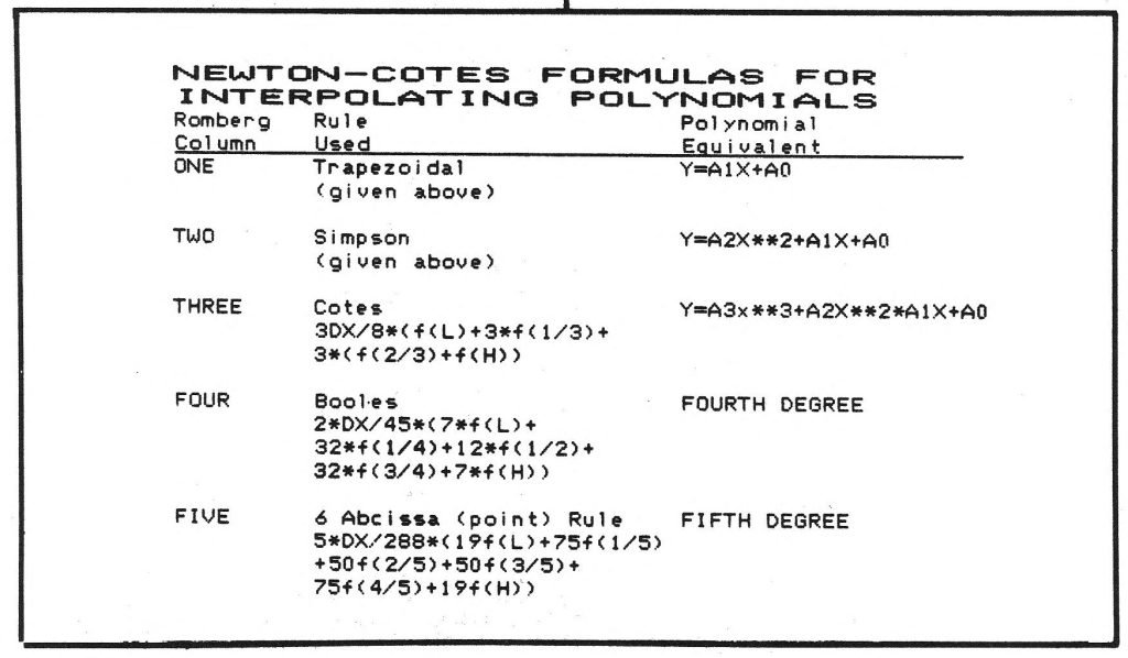
It turns out that Rombergs rule refines values INTERPOLATED by trapezoid boundaries. The more trapezoids, the higher the interpolation, as follows (see the second table for further clarification):

The error decreases by a factor of 4 for every step down col. 1, and 4**(N-1) as you go across (N=col no), S1 is 16 times more accurate than T1. B1 however has 6 decimal places better accuracy, and the 6 abscissa rule is better than 10 places, which is as good as you can do before truncation error takes over. B2 at 8 place accuracy should also give an exact answer. This system has some drawbacks that you should be aware of. First, your points must be spaced evenly and you need the right number of points in multiples + 1 of the degree you desire. For Simpsons rule (second degree), you need an odd number of points. For Cotes (third degree), you need 4, 7, 10, etc., points. This method is slow, but it is much faster than evaluating 128 trapezoids. For four iterations of Romberg, you need to evaluate 17 data points (2N+1). The first three iterations take about one to two seconds apiece to evaluate, the fourth takes about four. The Romberg correction to 128 trapezoids takes about another two seconds. 128 trapezoids goes into several minutes to evalute when summed independently.

If your points are unevenly spaced then interpolate it with SE and use VAL F$. The answer should be the same. Since integrating a particular function or set of data can be very specific and hard to generalize about, what follows is a table to pick specific equations from to help speed up your basic programming.

OK, now you’ve got several methods for evaluating polynomials, but the fastest way to get better than 6 decimal place accuracy requires about 10 seconds. A polynomial function can be integrated by sight or by hand that fast (if it’s an easy one). What if your equation is 1/X**2, and you need to integrate between 0 and 2? All the methods described fail. What if your equation has 5 variables and you need them all tested between 0 and 10? Oh, one more thing; you need all the answers in an hour. Well, don’t skip town because Gauss has done it again with:

This technique is the fastest and what I consider the best all around integration method. Up front though, there are disadvantages to this method. Unless you have a real time clock, discrete data points can’t take advantage of this method. You need a function. A dimension statement is required to hold the coefficients and weights, and the method is only good with functions whose limits are between -1 and +1. It is also very difficult to tell how much error is involved in your answer. As you take more points, you don’t approach your answer, instead you hit all around it (you may also hit right on it but not know it). This appears to severely limit the usefulness of Gauss Quadrature (GQ). In fact, GQ is the most widely used method because of its speed. We have advanced function development capabilities at our beck and call, We have room for a dimension statement, and now all we need is a method to transform any function to begin at -1 and end at +1.

Reasons for using GQ are the ability to integrate to infinite limits (provided the first point tested < 1e38) and SPEED, You can run through vast combinations variables, A*X**2+B*X+C, by putting A, B, C, and X in loops and calculating 3 or 4 integrals per second! In BASIC!

Now, the method to this madness (again no gory details). Using trapezoids, you need the first and last points. With Simpsons rule, you are required to have the mid-point as well. Gauss wanted a general way to evaluate some tough functions without going through 500 trapezoids to get better accuracy. Using simultaneous equations, he proved that as long as the limits were +/-1, any function evaluated where X =+-(1/SQR3), added up and divided by 2 would equal the area under the curve (up to third degree). That means evaluating two points to determine a cubic polynomial!

Implementing GQ is simple and straight forward, When evaluating from low (L) to high (H), DX = (HL)/2 and each X term evaluated must be converted to a relative position between +/-1 as if L =-1 and H =+1. This simple conversion is:

X' = ((H-l)*X+H+L)/2

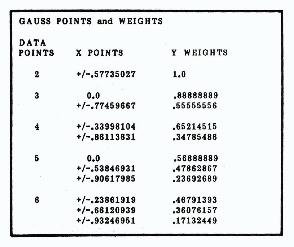
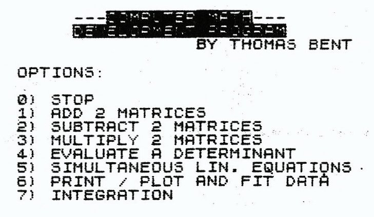
X, in this equation for two points, = (+/~) 1/SQR3 and X’ now becomes the new X. After this, eVALuate F$, multiply by the Y weighting factor, add them pup and multiply by DX and there you have it. (practically painless, isn’t it?) By the way, this is all done in TWO calculation lines. Another table of values is given to save you the trouble of looking for them. The program as listed, contains the coefficients and weights for 2, 3 and 4 points. The numbers look strange but are in accordance with the convention used in the SE program and can be incorporated quite easily. Add a 7. INTEGRATION at the main menu and at the plot menu with the appropriate GOSUB and RETURN. Believe it or not, but this simple routine is used on those big mainframe computers in analysis of bridges, aircraft, etc. Remember, Static (Strength of Materials) and Dynamic theory for structure evaluation evolved about the time of Gauss’ departure. Before this, those bridges collapsed a lot more often.

There are other methods used for integrating, including Monte Carlo, which generates RANDom numbers that either hit (below VAL F$) or miss (above VAL F$). This method is very slow. For 3 place accuracy, you need at least 4 orders of magnitude (10,000) evaluations of RAND and VAL F$. Leave this slow poke for the really fast mainframes. The text is short this time, but the routines are packed. Some good examples will be forthcoming, but I believe you can find lots of good applications for these routines. Next time, I will expose some Differentiation techniques that I hope you will find useful.

5997 REM INTEGRATION
5998 PRINT ,,"1) GAUSS QUAD",,"2) SIMP.-DATA",,"3) SIMP.-FUNC.",,"4) ROMBERG"
6000 INPUT Z
6001 FAST
6002 GOSUB (6060 AND Z=A)+(6500 AND Z=TW)+(6600 AND Z=TR)+(7200 AND Z=D)
6003 PAUSE 4E4
6004 GOTO 1000
6005 PRINT " INPUT FUNCTION? 1/0 NO=0"
6006 INPUT X
6007 IF X THEN INPUT F$
6010 PRINT "INTEGRATION",," INPUT START THEN STOP LIMITS"
6020 INPUT L
6030 PRINT L,
6040 INPUT H
6050 PRINT H
6051 RETURN
6060 REM GAUSS QUAD
6070 GOSUB 6005
6080 DIM S(TR,D)
6090 DIM T(TR,D)
6100 LET S(A,A)=A
6102 LET S(A,TW)=A
6104 LET S(TW,A)=(A+D)/(TR*TR)
6106 LET S(TW,TW)=(D+D)/(TR*TR)
6108 LET S(TW,TR)=S(TW,A)
6110 LET S(TR,A)=.65214516
6112 LET S(TR,TR)=S(TR,A)
6114 LET S(TR,TW)=.34785485
6116 LET S(TR,D)=S(TR,TW)
6120 LET T(A,TW)=A/SWR TR
6122 LET T(A,A)=-T(A,TW)
6124 LET T(TW,TR)=SQR (TR/(D+A))
6126 LET T(TW,A)=-T(TR,TR)
6128 LET T(TR,TR)=.33998104
6130 LET T(TR,A)=-T(TR,TR)
6132 LET T(TR,D)=.86113631
6134 LET T(TR,TW)=-T(TR,D)
6135 PRINT " INPUT NO. OF POINTS 2<=>4"
6136 INPUT DEG
6140 LET DX=(H-L)/TW
6142 LET FZ=ZO
6150 LET K=DEG-A
6160 FOR I=A TO DEG
6180 LET X=((H=L)*T(K,I)+H+L)/TW
6190 LET FX=FX+S(K,I)*VAL F$
6210 NEXT I
6220 LET FZ=FZ*DX
6230 PRINT "GAUSS QUAD= ",FX
6250 RETURN
6501 REM SIMPDAT
6510 LET FZ=ZO
6520 LET DX=U(TW)-U(A)
6550 FOR I=A TO DP-TW STEP TW
6560 LET FX=FX+DX/TR*(Y(I)+D*Y(I+A)+Y(I+TW))
6570 NEXT I
6590 PRINT "SIMPSONS AREA = ";FX
6599 RETURN
6600 REM SIMP FUNC
6610 GOSUB 6005
6630 PRINT " INPUT MAX ITERATIONS.(<=8)"
6635 INPUT IT
6640 CLS
6650 FOR I=1 TO IT
6660 LET DIV=2**I
6670 LET AR=ZO
6680 LET DX=(H-L)/DIV
6683 LET T=DX/TR
6690 LET SIM=DIV/TW
6700 FOR J=A TO SIM
6705 LET FZ=ZO
6720 LET X=L+TW*(J-A)*DX
6725 LET FX=VAL F$
6730 LET X=X+DX
6732 LET FX=FX+4*VAL F$
6735 LET X=X+DX
6740 LET AR=AR+(FX+VAL F$)*T
6810 NEXT J
6820 PRINT " FOR ";DIV;" DIVISIONS, AREA=",AR,,
6830 PAUSE 50
6835 IF Z>TR THEN RETURN
6840 NEXT I
6900 RETURN
7200 REM TRAPEZOID RULE
7210 GOSUB 6005
7300 PRINT " INPUT MAX ITERATIONS. (<=6)"
7310 INPUT IT
7320 DIM A(IT,IT)
7325 CLS
7330 FOR I=A TO IT
7340 LET DIV=TW**(I-A)
7350 LET AR=ZO
7360 LET DX=(H=L)/DIV
7365 LET T=DX/TW
7370 FOR J=A TO DIC
7375 LET FZ=ZO
7380 LET X=L+(J-A)*DX
7390 LET FX=FX+VAL F$
7400 LET X=L+J*DX
7410 LET AR=AR+(FX+VAL F$)*T
7420 NEXT J
7425 LET A(I,A)=AR
7430 GOSUB 6820
7450 NEXT I
7500 REM ROMBERG METHOD
7305 CLS
7530 FOR J=TW TO IT
7535 LET T=D**(J-A)
7540 FOR I=J TO IT
7560 LET A(I,J)=(T*A(I,J-A)-A(I-A,J-A))/(T-A)
7570 NEXT I
7580 NEXT J
7585 SLOW
7590 FOR I=A TO IT
7595 PRINT
7600 FOR J=A TO I
7610 PRINT A(I,J);"  ";
7620 NEXT J
7625 PRINT
7630 NEXT I
7640 FAST
7650 RETURN

Finally, the last thing on my agenda for this volume is the documentation for the program. Please, read the annotations! There is a lot of information in the listing itself. I know of more than one person who “gritted their teeth” and drank a lot of coffee, and succeeded in entering the listing by hand. They truly wanted to LEARN this fine art. I have not included a flow chart or a listing of variables, however many are defined in the listing. If you make a working copy, then most initialization and quadrature LET statements can be left out. I also did not assign subroutines to variables, for example, GOSUB 1760, could be GOSUB GE, if you LET GE=1760. This would be even more of a savings on space, Making the PLOT arrays into string arrays would create a whopping big space savings. If you have a few hundred data points and you really want to manipulate them (in 16K), then this may be a necessity.

What started out to be a small, quick and dirty method of viewing data, blossomed into a rather fine, option driven plot program (in amongst all the other things this program will do). Plotting and fitting data, applies virtually every aspect of what we have covered here and quite a bit more.

This program makes rather extensive use of arrays (keeps computation loops simple), and you really don’t have to worry about losing your data by mistake. If you have a lot of data (more than 70 points) then you may need more than 16K. Basic flags are used to keep track of what is going on in the subroutines, and “Z” is used for screen dumps. Although array plotting is not memory efficient, it is considerably faster than plotting and calculating at the same time. With the ability to recall data or functions, rescale and refit, you have flexibility not typical of many ZX/TS programs. A sample senario follows:

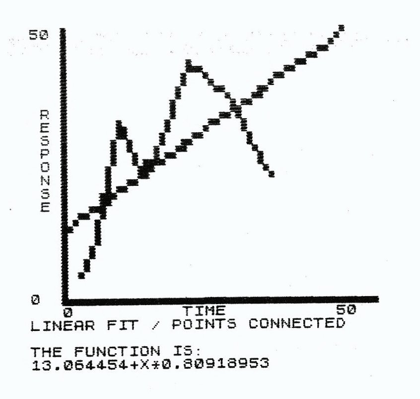
1. LOAD “SE”, When the main menu appears, press 6 (to input data for plotting). “How many data points?” will appear. Give a number and then enter X and Y values in pairs. Printing is done after each pair. Next, the menu asks, “Whay would you like to do?” You MUST plot your data first (choice 1). This will set the parameters for scaling. (This is done to save space. You could initialize all these flags to zero and set screen size around line 1000 if you want.) You need never label your graph or give it a name until your ready to COPY. Set your scale (LIN/LOG) and set your limits (LOW/HIGH) for graphing. This is only necessary on the first plot. These values are retained until you change your graph limits. Connect your points at any time (this is a screen function), but only plot a curve fit after you have fit it (2 and 3).
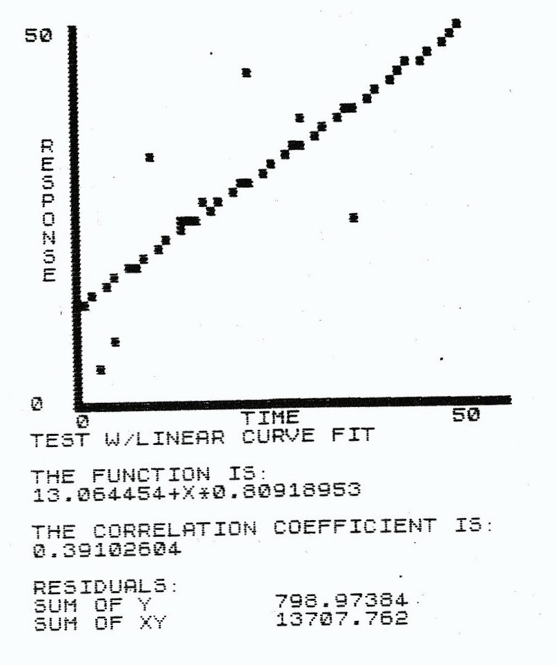
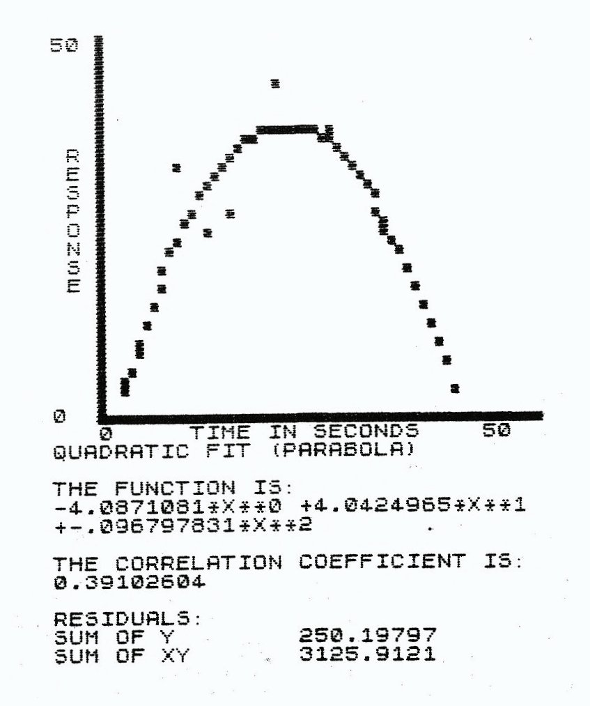
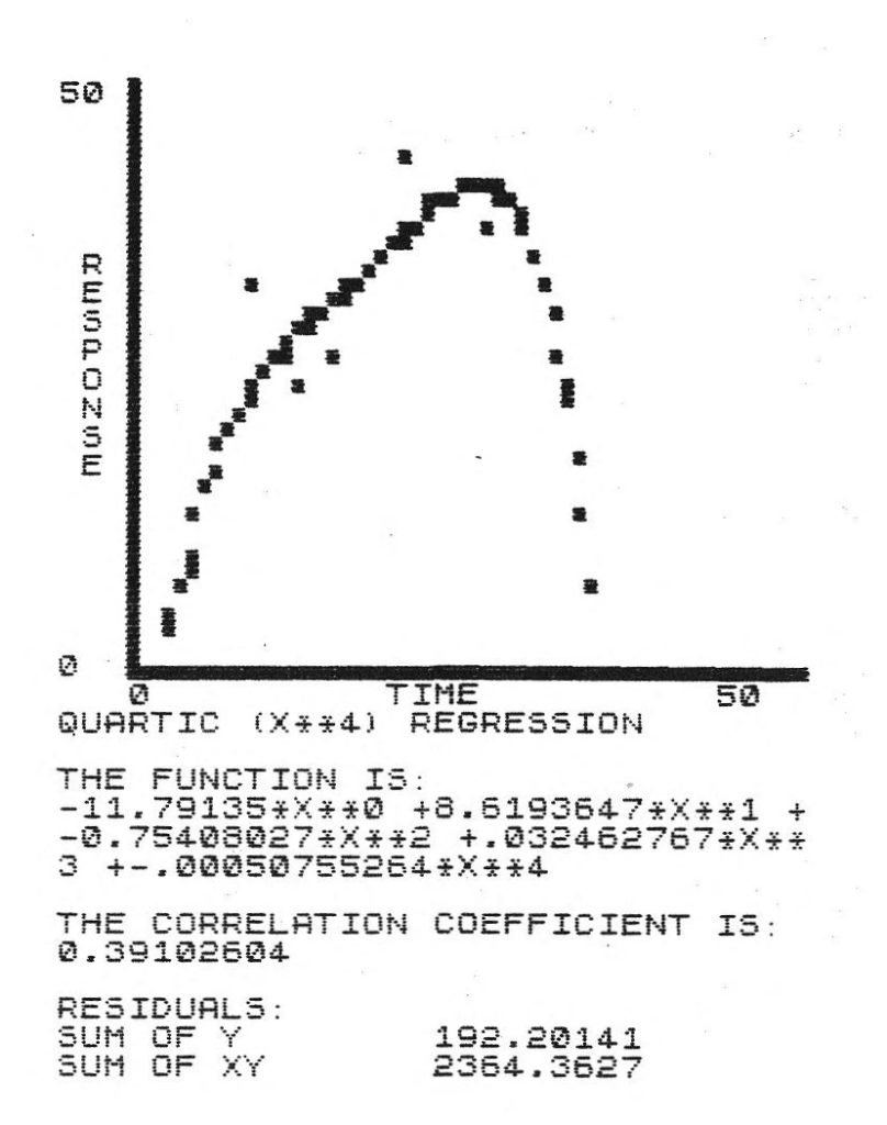
2. Fitting the data comes next (choice 2). Notice on the various screen dumps, just how many ways you can fit the same data points. All of the graphs are of the same set. Remarkable, isn’t it? There are so many possibilities here that I couldn’t come close to naming them. You have four linear regression, any size interpolation (each degree is different) and polynomial regression to choose from. Just experiment until you get a good fit (part of the learning curve). Remember, no negative values or zero for any data in linear regression except linear (LIN/LIN on both X and Y axes) itself.
3. Scale your choice of fit if you wish to plot it (choice 3). This routine was separated from the fit routine, to accomodate the interpolation routine shortcomings. They are not really shortcomings, because interpolation is done in small pieces. For example, if you have 10 data points to interpolate, then (look back at the form for interpolating polynomial) there will be a X**9 term in every equation. You are losing accuracy at a very fast rate. You are much better off taking them three or four points at a time. Unless you have a very good system of points, then you will probably get an error B, integer out of range error, with a large interpolation, so be careful!
   
   Input your start and stop values for the X axis, This is the area to pay attention to if you are interested in forecasting and trend prediction. Leave enough “headroom” and specify the screen limits, and your ZX computer will plot your trends. Input the desired point density (the number of points to be plotted on the screen, 40 is pretty good) and let it run for about 20 seconds.
4. You will be back at the plot menu now. This time, when you plot your graph, specify curve fit and see your results. The curve statistics will be lprinted if you press “Z.”

If you rescale your graph, then rescale your fit.

Choice four will bring you to the print menu. If you desire Iprinting, then add an Iprint line where it is required. You may print from your data (and correct it in the direct mode), your curve or any other curve you can think of. When using interpolation, if you specify all of your data, and the degree of fit versus the number of data points DON’T match, then you will be asked if you would like a listing as plotting multiple interpolations is not implemented. More programming is required to implement this capability.

If you go back to the main menu (choice zero), then you can go out to the integration subroutine. Pick your choice of routines and set your integration limits. If you do not want to input a new function, then enter zero (0) when asked. When finished, you will go back to the main menu. If you care to plot the same points again, then STOP (0) and GOTO 666. This will bring back the PLOT menu.

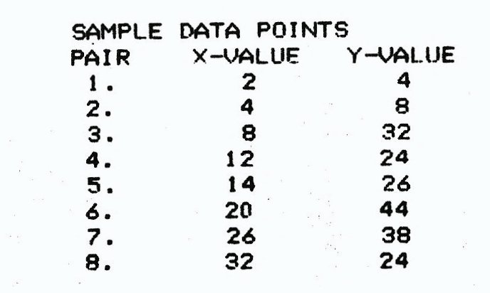
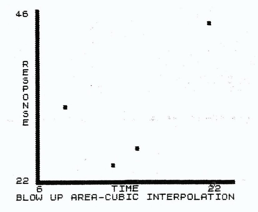
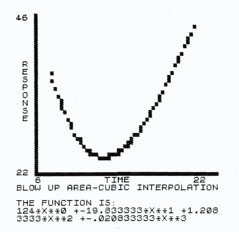
To give you an idea of the power of SE, I have listed some of the menus available. I input a short table of data, plotted it and fit it with several different curves. You can rescale and enlarge an are if you want. My enlargement is fir with a cubic interperpolating polynombial. Boy, what a good fit!

The data for each graph is identical. Only the curve fit has been changed in each case.