Math Development Program, Part 2

Ok, Ok, I can hear it now; it’s just another simultaneous equation program. Anybody can write one or at least find one in a good computer math book (they seem to be proliferating these days), besides what good are they anyway? I’d now like to present Part 2 in a continuing series; but first, let’s hear it for Gauss. I mean really! The man died in 1855 and did for math (and physics) what Newton did for figs (and apples). I don’t think pencils had been invented in his time, but he still managed to figure out all of these relationships. Well, enough reminiscence already. The first of three routines up for examination will be “Interpolating Polynomial.” This will be followed with Polynomial Regression (Least Squares) and end with a few words on plotting. Along the way we shall touch on a few interesting (I hope) topics which some knowledge of will help demystify this area of math.

This first routine “INTERPOLATES” (as opposed to extrapolate) or calculates values IN BETWEEN known values with the EXACT and only polynomial of the given (Nth) degree that fits the given (N+1) points. The polynomial is unique and independent of the method used to find the equation. This means that regardless of which method you use, the answer should be the same. Beware of roundoff error however. If you compare the results of the SE routines, you can see minor differences from time to time. Since the Interpolating Polynomial deals with definite values (must be a function of X), it will find an exact solution (not withstanding roundoff error). A check on ill-conditioning may show a very ill-conditioned system of equations. This is due in part to manipulating both large and small numbers in the same system creating a truncation error as well as roundoff error.

As the section on fitting goes, I suppose we should start at square one (or should I say, line one); The Straight Line Subroutine. You can find one in your TS/ZX manual, or a better one in the first issue of SWN. Alright, so what does it do? You might say it plays the percentages. If Y = f(X) and you would like to know what Y is between two known X values, the equation is:

Y(low)+(X-X(low))/(X(top)-X(low))*(Y(top)-Y(low)

Or, in other words, the percentage of the X value above X(low) times the range of the Y values. Put X in a loop from X(low) to X(top), and you will have a tabular, linear interpolation printout. Plotting is slightly tougher though. We have incorporated a compacted version of the Straight line subroutine in the main programs’s plot routine. This code checks the slope of the line and then steps between the X values for slopes less than one and steps between the Y values for slopes greater than one. Just make sure your values are on scale first.

Linear interpolation is fine for some applications (such as plotting on the coarse TS/ZX pixels), but is usually only accurate for very small distances away from the known point. To get a better approximation of values between two points, it would be nice to fit the points with a higher order function – say a parabola. Since two points define a particular line, we need a little more information for a parabola. How about three points. A unique parabola is defined by 3 points, a cubic by 4 and so on… You now have the power to fit any number of points that you specify. Don’t get too carried away, or the results you get will be worthless.

The interpolation subroutine loads the array in A so as to set up the required number of equations for the given number of points. The equations are Polynomial, of course, but please take note of the method used to generate the equations. Yes, in case you hadn’t noticed, more loops. One difference you will see is that the array is filled backwards and an arbitrary constant term is used to help facilitate filling the array as well as validate our polynomial. One, is always a nice number for a constant and is used here. This method is a tremendous memory saving method over any other I know of that will generate any size polynomial. For you fanatics out there, the X determinant is called a Vandermonde determinant. There are other methods, of course, that you can use to solve this type of problem.

These methods of interpolation include Lagrange, which solves a determinant; Aitken’s, which takes Lagrange for many points and tells you which degree fit, fits the most points; and Newton’s forward and backward difference methods (same guy that invented figs), to name a few. Newton’s method is a little beyond our scope here, but it is a widely used method for trying to get a handle on error involved in interpolation. Its device is to interpolate in small steps from one or both ends and therefore reduce error. You must know a lot of points first though. This is a good method for plodding through large tables of data which you must fill in accurately inbetween values (eg., log tables). This method is used by monks and masochistic bosses of high degree.

I would at this time like to spend a few moments deriving Lagrange’s method, since it pertains directly to part one of this series. Let’s develop our determinant: for a first degree polynomial. This method won’t give a function per se, but it will evaluate a table of data to any degree that we care to program for.

Let’s start with the equation Y = MX + B (straight line) where Y is the value we’re after, and X is the number we will plug and chug with. B is a constant (Y-intercept) and M, of course, is the slope of the line, We’ll let A0 = B, A1 = M and Y = P(X). We need to know a point before and after X, called X0 and X1. Their Y coordinates respectively shall be, f(X0) and f(X1). We must also define a constant K = 1, to initialize our array. As we plod through our calculations, this constant more or less retains a space for our Y-intercept (A0) in the determinant.

If Y = MX + B then
P(X) = A1X + A0 therefore:
P(X) = A1X - A0 = 0
and by the same reasoning,
f(X0) - A1X0 - A0 = 0
f(X1) - A1X1 - A0 = 0

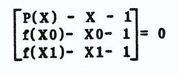
Since it is a straight line, all of the equations have the same slope A1, and Y-intercept AO. If the points are real (as opposed to contrived), then there is a non-zero determinant of the coefficients, as follows:

At this point, I refer you to the Part one section on determinants to achieve the following expansion along the first column and solve for P(X):

P(X)=f(X0)*((X-X1)/(X0-X1))+f(X1)*((X-X0)/(X1-X0))

All values are given except P(X), and X should be a loop counter between X0 and X1. The following program calculates all determinant (det) values first, and then it multiplies each det with its associated Y value and adds them up. Higher degree solutions look like this:

Second degree (3 points)

Det0 = ((X-X1)*(X-X2))/((X0-X1)*(X0-X2))
Det1 = ((X-X0)*(X-X2))/((X1-X0)*(X1-X2))
Det2 = ((X-X0)*(X-X1))/((X2-X0)*(X2-X1)) 

P(X) = f(X0)*Deto + f(X1)*Detl + f(X2)*Det2

There is a conspicuous pattern that develops with the X’s. You can interpolate to any degree your little heart desires by following it. What follows is a little program to calculate a sine table by third degree interpolation. Remember that the ZX/TS uses a radian mode, so to compare you must convert actual sine values to degrees. We will cover this program a little more later on when we talk about error.

1 REM SINE INTERPOLATION
5 LET X0=0
10 LET FX0=0
15 LET X1=30
20 LET FX1=.5
25 LET X2=60
30 LET FX2=.8660254
35 LET X3=90
40 LET FX3=1
44 SCROLL
45 PRINT "DEG. LAGRANGE     TRUE SINE"
46 SCROLL
50 FOR X=0 TO 90 STEP 10
60 LET DET0=((X-X1)*(X-X2)*(X-X3))/((X0-X1)*(X0-X2)*(X0-X3))
70 LET DET1=((X-X0)*(X-X2)*(X-X3))/((X1-X0)*(X1-X2)*(X1-X3))
80 LET DET2=((X-X0)*(X-X1)*(X-X3))/((X2-X0)*(X2-X1)*(X2-X3))
90 LET DET3=((X-X0)*(X-X1)*(X-X2))/((X3-X0)*(X3-X1)*(X3-X2))
100 LET PX=FX0*DET0+FX1*DET1+FX2*DET2+FX3*DET3
110 LET Z=SIN (X/180*PI)
120 SCROLL
130 PRINT X;TAB 5;PX;TAB 18;Z
140 NEXT X
150 STOP
160 SAVE "SINE"
170 RUN

“Boy! I just used an interpolating polynomial to fit some data points, and got the wierdest plot! It can’t possibly be correct?” While an interpolating polynomial gives an exact equation that goes through every point, those points may not, and probably will not, lie at the maximum or minimum values. It is possible to interpolate a group of data of which two points have coordinates of say, (4,5) and (6,9), with a maximum value in between, such that when X = 5, Y may equal 100 or even 1,000,000! This is slightly ill-conditioned to say the least. If you interpolate 8 points then you may have as many as 7 max or min values to contend with. Is there a better way? Well, maybe. You shall be the judge and jury.

200 REM LEAST SQUARES
210 PRINT " INPUT NO. OF DATA POINTS"
220 INPUT N
222 DIM X(N)
224 DIM Y(N)
230 SCROLL
240 PRINT "NO  X","Y"
250 FOR I=1 TO N
260 SCROLL
270 INPUT X(I)
280 INPUT Y(I)
290 PRINT I;TAB 4;X(I),Y(I)
300 NEXT I
310 LET A=NOT PI
320 LET E=A
330 LET C=A
340 LET D=A
350 FOR I=1 TO N
360 LET T=X(I)
370 LET TY=Y(I)
380 LET A=A+T
390 LET E=E+T*T
400 LET C=C+TY
410 LET D=D+T*TY
430 NEXT I
450 REM CRAMERS RULE
460 LET CR=N*E-A*A
470 IF NOT CR THEN STOP
480 LET B=(C*E-A*D)/CR
490 LET M=(N*D-C*A)/CR
500 CLS
510 PRINT "THE FUNCTION IS:",,,
520 PRINT "Y=";M;"*X + ";B

Least Squares method of curve fitting is another widely used method of curve fitting that will give a smooth fit through a lot of data. If your data is approximate or downright inaccurate, then this method is for you. In contrast to an interpolating polynomial, you get a smooth curve that may not touch any of the given values.

Why call it least squares? Let’s go back to our main man, Gauss, again. He wanted a method to fit much collected, ambiguous data smoothly, and deduced that squaring all terms would eliminate all negatives that may cause an inverted fit (probably found out the hard way). An inverted fit is one where all of the points are opposite in sign from your data. Second, call it Least Squares because the object is to have the sum of the Squares of the differences between the actual values and the fitted values to be as small as possible (Oh Yes! more statistics!), Smooth curve? Fit approximate data? Sounds great, but just what is needed to make this technique work? To start with, a sound, sober analytical mind that can eyeball data and deduce the right equation for the function without all this hulla~ballou. A trifle too much to ask for probably, but thank God for Gauss and 2X/TS’s.

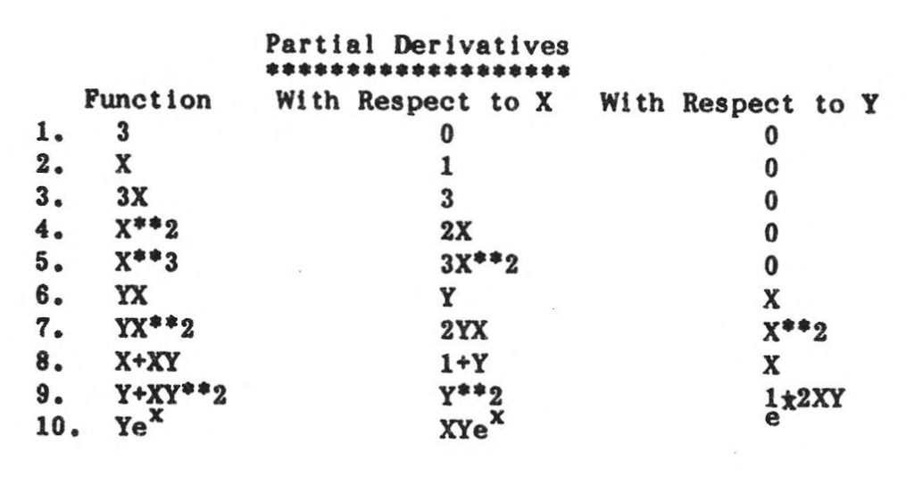
Now, I find it necessary to digress (hopefully evolve for some) momentarily, to cover some background to help in general, the understanding of smooth curve fitting, and in particular, the next few paragraphs as we derive a least squares routine. This subject brings shudders and heart murmurs from those who know about them, but for those of you who don’t, have no fear as there is nothing to be afraid of. Now, a few words about Partial Derivatives. This won’t substitute for a good Calculus 3 class, but it may alleviate possible ambiguities that may arise. The best way I know how to describe them is with a table. Please examine the following:

Very simply, the derivative of a constant is zero. If you “freeze” a function in time or space (values are not changing), then a variable with respect to another variable is a constant. At this point, the partial is solved like a normal derivative. As a rule of thumb, if you have a function with more than one variable type (Z = f(X,Y)), it is easier to work with two partial derivatives (lines) than it is to work with the function as a whole (variable surface in 3-d). This is especially true in computer programming. Visualizing a surface and programming for it are two entirely different things.

So, what do partial derivatives have to do with the price of tea in China? Not much. Computer curve fitting in general does require solving partial differential equations with respect to each “Degree of Freedom” to determine a curve fit. The degrees of freedom are basically the constants that describe the coefficients for the function in question.

If f(X) = A1X + AO, then A1 and A0 are the coefficients to be solved for and we have two degrees of freedom. We will proceed and derive a linear least squares, but don’t worry, we have our subroutines for handling this stuff already, thank Gauss!

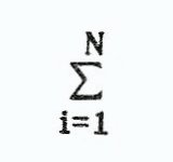
What is needed for us to make our Least Squares fit? Well, at first glance, we want the fit line as close as possible to all of our points, or, the calculated Y values minus the actual Y values equal to zero. These values are called the Residuals, Least Squares criterion is actually all of the residual terms squared and added up. You may ask if there is an equation for this, but be patient, it’s coming. We have one more term to cover before we proceed, this being the signum or summation notation. This means the sum of all the following terms from a starting value to Stopping value say, i = 1 to N, but it sounds like grounds for a loop to me. You will see this written in text books as follows:

N in this expression will be the number of data points we provide.

Let’s finally get back to the mainstream and our fundamental equation, Y = MX + B, or in our case f(X) = A1X + AO. The least square equation for a linear fit is:

Since Y(calc.) = f(X) = A1X + A0, a direct substitution may be made into the above equation for R (sum of the residuals), We now set the partials of R with respect to each constant to zero and solve two linear simultaneous equations (easy since we’re all experts now). The partials of R with respect to:

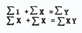
The 2’s are in all terms and therefore drop out. Multiplying the second equation through by X and moving the Y(i)’s to the other side, gives the following system of equations:

AO and A1 are coefficients to be determined by the computer and are initialized to one (that marvelous constant giving a helping hand once again), This leaves a simpler system still with which we must manage:

Since we are adding up the values for each X and Y term, the Zi term becomes the number of data points that are input. This system gives us a good use for Cramer’s rule; Least Squares Linear Regression. Now the answer for that question, what do we need for a least square fit?

1. The number of data points.
2. The sum of the X terms.
3. The sum of the Y terms.
4. The sum of the X*Y terms.
5. The sum of the X**2 terms.
6. One Cramer’s rule subroutine.

This system assumes that the X values are more accurate than the Y values. If they’re not, then Swap your X and Y terms to improve your fit. This method of fitting may be used to fit many different types of equations. Logarithmic, Exponential and Power fit methods all use this system of equations to find their solutions. What’s the difference? How the data is manipulated before you sum your variables. These methods simply take the natural log (In) of the X or Y or both before they are summed. REMEMBER!! The LN of Zero and Negative numbers are undefined and not allowed (program will stop). This leaves only one linear method, to fit data with values less than or equal to zero. Keep in mind that there are as many ways to fit data as there are pixels on the screen, so don’t let a bad fit using one method stop you from trying some other method (memory permitting). With a little knowledge of statistics and enough degrees of freedom you can fit your data. It just requires a function and partial derivatives for each coefficient (no fun, but true none-the-less).

If your data appears to resemble a polynomial of some degree, then you might try our nifty little polynomial regression routine, Actually, it is the same routine as the linear regression, but uses the interpolation routine to derive a function. You may derive as high a degree of fit as your memory dictates, the routine creates an array (C) to fill array A, and then deletes array C when it is finished. Since not all of you have extravagant amounts of memory to play with, I have a more conventional linear least squares routine following this. It does the same thing as the one in the main program, but is easier to follow. Most programs on the market use this approach. Try cubic regression and see how memory efficient it is (needs Gauss elim. to solve).

At this point, I would like to recap briefly what we have covered. First, the simultaneous equations and their derivation. Second, interpolation in general, with a derivation of the LaGrange polynomial and a few words about the straight line subroutine. Third, Least Squares curve fit with a linear derivation and a few words about partial derivatives.

These routines are fairly easy to derive and implement, but what about higher orders of magnitude? How do the equations compare? What does the computer see? Are the results accurate? Even better, will your boss believe you if you tell him you did it on a ZX/TS rather than an IBM mainframe?

First, my opinion on the last question; if you boss starches his collar, then don’t tell him right away that a TS1000 solved his problem. Show him the good work first. As for the other questions, let’s compare quadratic interpolation and quadratic regression and look at what the computer sees. The two routines, Interpolating Polynomial and Polynomial Regression, are not easy to follow (just try some other way to get all that in 16K), albeit there are relatively few calculation lines. Triple loops have a habit of concealing vast amounts of computation in a few (even one) calculation lines. Interpolation uses a double loop for initializing Y values and setting all X values to one, a triple loop to build the X determinant into its higher order (backwards, from right to left) and a single loop to switch the coefficients back around on returning from the Gauss elimination subroutine.

Along the same lines, the regression routine uses a single loop to initialize column one of array C to one, a double loop to load and build array C with X values, a triple loop to load array A with array C values and further build array A and a double loop to load the last column of A with the sums of the Y values * the first column of X values from array C. (Remember, column 1 of C started with all ones.)

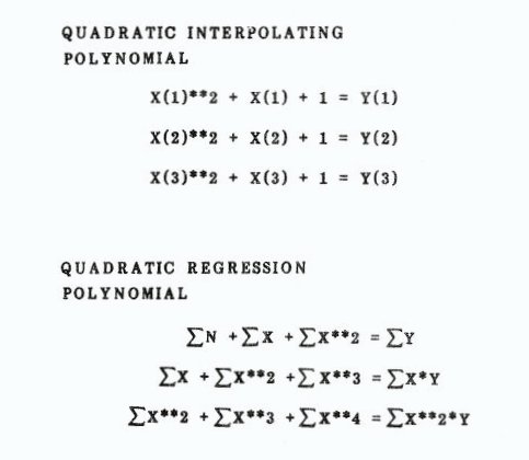
Here are the equations and systems we are solving for:

As you can see, the equations are quite polynomial, and follow a clear pattern of development. This makes any degree polynomial relatively easy to program (memory permitting).

The difference between linear and quadratic interpolation is column 1 and row 3; for regression is column 3 and row 3. Remove these rows and columns from the system and you have the linear form. The computer sees only array A in its computation (dynamically dimensioned as needed as DIM A(M,N)), necessitating a lot of loops to fill it (loops keep the program length down).

Error, on the other hand, is not so easy to get a handle on. Fortunately, Least Squares negates the effect of error by running an average line through all of the data points, acknowledging that every data point may be inaccurate. The residuals should equal zero (the sum of the f(X)-Y values, also the X*(f(X)-Y) values. These statistics may be checked after F$ has been calculated in the program. Linear regression can be checked for goodness of fit by using the Pearson Product Moment Correlation Coefficient, easily and efficiently by adding up all the Y squared terms as well (Y2). A perfect fit =1; good =>.8, This term is not of much value for higher orders of fit.

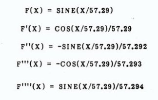
Interpolation is supposed to give an exact equation, but I’m sure you all know better by now. (I hope so anyway.) Look to the N+1 derivative of the function for the error solution. If you have a third degree Polynomial, then look at the fourth derivative. Say WHAT!! Did I hear you say that the fourth derivative of a third degree polynomial is ZERO? You whizzes are really on the ball out there, It is an EXACT polynomial, right? Well, let’s take another look at the sine interpolation demo. The fourth derivative of sine is still sine, and it is not zero. Because the computer calculates in radian mode (1 Radian = 57.29 degrees), the conversion to meaningful numbers is made. Examine the following terms:

If the maximum value for sine is one (90 degrees), then 1/57.29**4 is the largest term that the fourth derivative can equal. To determine the maximum error, determine the difference between all known data points and the value at which you want to determine the error at. Multiply that by the max error and divide by N factorial (N=power of the derivative you are looking at; 4 in this case). For the sine of 10 degrees, the maximum error can be no larger than:

1/57.29**4 * (10*-20*-50*-80)/(4*3*2*1) = -3.1E3

The accuracy is better than two decimal places at worst. This calculation is comparible is the remainder term of a taylor series (another bag of worms), When you reach a given value of X, then a zero enters the equation and the error term of course becomes zero and drops out (watch out for roundoff error. Since we know a few of the terms (even smaller than 1), then we know that the error is less. This also indicates that the error is larger as we approach 90 degrees. Have fun with this one!

4000 REM PRINT VALUES
4010 PRINT "WOULD YOU LIKE TO PRINT FROM:",,,"0. INPUT DATA",,"1. CURVE FIT",,"2. OTHER FUNCTION"
4020 SLOW
4030 INPUT Z
4040 GOTO (4050 AND NOT Z)+(4140 AND Z=1)+(4120 AND Z=2)
4050 GOSUB 910
4060 PRINT "NO. X","F(X)"
4070 FOR I=1 TO DP
4080 GOSUB 910
4090 PRINT I;TAB 4;P(I),Y(I)
4100 NEXT I
4110 GOTO 4300
4120 PRINT " INPUT F(X)"
4130 INPUT F$
4140 PRINT " INPUT X START";
4150 INPUT XS
4160 PRINT XS
4170 PRINT " INPUT X STOP";
4180 INPUT XP
4190 PRINT XP
4200 PRINT " INPUT STEP VAL "
4210 INPUT INC
4220 CLS
4230 IF LS OR Z THEN PRINT AT 16,D;"THE FUNCTION IS:",F$
4240 GOSUB 910
4250 PRINT "X","F(X)"
4260 FOR X=XS TO XP STEP INC
4270 GOSUB 910
4280 PRINT X,VAL F$
4290 NEXT X
4300 GOSUB 910
4309 POKE 16418,0
4310 PRINT AT 21,30;," INPUT ANY KEY-""Z"" TO COPY "
4320 PAUSE 4E4
4330 FAST
4340 IF INKEY$="Z" THEN COPY
4350 IF LS THEN RETURN
4360 LET M=DP
4370 LET AL=ZO
4380 LET LS=ZO
4390 RETURN
4400 REM INTERPOLATING POLYNOMIAL
4410 PRINT " INPUT POSITION, IN ORDER OF","ENTRY, OF THE FIRST X TERM TO BEEVALUATED"
4420 INPUT POS
4430 PRINT ,,"DO YOU WANT TO FIT THE REST OF  THE POINTS? YES=1 NO=0"
4440 INPUT AL
4450 IF AL THEN PRINT "YOU CANNOT PLOT DIRECTLY.","WANT A LIST?YES=1 NO=0"
4460 IF NOT AL THEN GOTO 4500
4470 INPUT LS
4480 PRINT " INPUT STEP VAL "
4490 INPUT INC
4500 FAST
4510 LET POS=POS-A
4520 LET LAST=POS+DEG
4530 IF LAST>DP THEN LET DEG=DP-POS
4540 LET M=DEG
4550 LET IP=PI
4560 LET N=M+A
4570 DIM A(M,N)
4580 FOR I=A TO M
4590 LET A(I,N)=Y(I+POS)
4600 FOR J=A TO M
4610 LET A(I,J)=A
4620 NEXT J
4630 NEXT I
4640 FOR J=M-A TO A STEP -A
4650 LET DE=DE+A
4660 FOR I=A TO M
4670 FOR K=A TO DE
4680 LET A(I,J)=A(I,J)*P(I+POS)
4690 NEXT K
4700 NEXT I
4710 NEXT J
4720 LET DE=ZO
4750 LET L=M
4760 FOR I=A TO M/TW
4770 LET T=X(I)
4780 LET X(I)=X(L)
4790 LET X(L)=T
4800 LET L=L-A
4810 NEXT I
4820 LET F$=""
4830 FOR I=A TO M
4840 PRINT "X";I;" = ";X(I)
4850 LET F$=F$+STR$ X(I)+"*X**"+ STR$(I-1)+" "
4860 IF I<>M THEN LET F$=F$+"+"
4870 NEXT I
4880 IF NOT AL THEN GOTO 5486
4890 LET XS=P(POS+A)
4900 LET XP=P(LAST)
4910 SLOW
4920 GOSUB 4230
4930 LET POS=LAST
4940 IF POS=DP THEN GOTO 4360
4950 CLS
4960 GOTO 4500
4980 REM LEAST SQUARES FIT
4990 CLS
5000 FAST
5010 FOR I=A TO M
5020 IF Z=A OR Z=TW OR Z=A+D THEN LET U(I)=P(I)
5030 IF Z=TR OR Z=D AND P(I)>ZO THEN LET U(I)=LN P(I)
5040 IF Z=A OR Z=TR OR Z=A+D THEN LET V(I)=Y(I)
5050 IF Z=TW OR Z=D AND Y(I)>ZO THEN LET V(I)=LN Y(I)
5060 NEXT I
5080 REM REGRESSION AREA FILL
5090 IF Z AND Z<A+D THEN LET DEG=TW
5100 LET M=DEG
5110 LET N=M+A
5120 DIM A(M,N)
5130 DIM C(DP,M)
5140 LET Y2=ZO
5150 FOR I=A TO DP
5160 LET C(I,A)=A
5170 LET Y2=Y2+V(I)*V(I)
5180 NEXT I
5190 FOR J=TW TO M
5200 FOR I=A TO DP
5210 LET C(I,J)=C(I,J-A)*U(I)
5220 NEXT I
5230 NEXT J
5240 FOR I=A TO M
5250 FOR J=A TO M
5260 FOR K=A TO DP
5270 LET A(I,J)=A(I,J)+C(K,I)*C(K,J)
5280 NEXT K
5290 NEXT J
5300 NEXT I
5310 FOR I=A TO M
5320 FOR J=A TO DP
5330 LET A(I,N)=A(I,N)+C(J,I)*V(J)
5340 NEXT J
5450 NEXT I
5360 DIM C(A)
5370 REM PEARSON PROD.MOMENT
5380 LET R=A(TW,N)-(A(TW,A)*A(A,N))/DP
5390 LET R=R*R
5400 LET R=R/(((A(TW,TW)-(A(TW,A)*A(TW,A))/DP)*(Y2-(A(A,N)*A(A,N))/DP)))
5410 LET IP=A
5420 GOSUB (2660 AND M=TW)+(1750 AND M>TW)
5430 LET IP=ZO
5440 IF M>TW THEN GOTO 4820
5450 LET F$=""
5460 IF Z=A THEN LET F$=STR$ X(A)+"+X*"+STR$ X(TW)
5470 IF Z=TW THEN LET F$=STR$ X(A)+"+X*"+STR$ X(TW)
5480 IF Z=TR THEN LET F$=STR$ X(A)+"+LN X*"+STR$ X(TW)
5485 IF Z=D THEN LET F$=STR$ (EXP X(A))+"*X**"+STR$ X(TW)
5486 REM RESIDUALS
5487 LET RXY=ZO
5488 LET RY=ZO
5489 FOR I=1 TO DP
5490 LET X=P(I)
5491 LET Y=Y(I)
5492 LET T=VAL F$
5495 LET RY=RY+(T-Y)*(T-Y)
5496 LET RXY=RXY+X*(T-Y)*(T-Y)
5498 NEXT I
5500 CLS
5510 PRINT "THE FUNCTION IS:",F$
5520 IF Z THEN PRINT "CORRELATION COEFFICIENT:",R
5522 IF Z THEN PRINT ,,"RESIDUALS",,"Y\'S",RY,"XY\'S",RXY
5530 GOTO 4309
5540 REM SCALE PLOT FIT
5550 PRINT " INPUT START VAL FOR X FIT"
5560 INPUT XS
5570 PRINT " INPUT STOP VAL FOR X FIT"
5580 INPUT XP
5590 PRINT ,," INPUT CURVE FIT POINT DENSITY"
5600 INPUT PD
5610 FAST
5620 LET K=LN 10
5630 GOSUB 146
5640 IF NOT XL THEN LET TXE=E(A)
5650 IF NOT YL THEN LET TYE=E(TR)
5660 IF XL THEN LET TXE=LN E(A)/K
5670 IF YL THEN LET TYE=LN E(TR)/K
5680 LET PF=A
5690 DIM F(PD+A)
5700 DIM G(PD+A)
5710 LET DF=(XP-XS)/PD
5720 FOR X=XS TO XP STEP DF
5730 LET FX=VAL F$
5740 IF FX<E(TR) OR FX>E(D) THEN GOTO 5860
5750 IF NOT XL THEN LET TX=X
5760 IF XL THEN LET TX=LN X/K
5770 IF YL THEN LET FX=LN FX/K
5780 LET TX=(TX-TXE)/DX
5790 LET FX=(FX-TYE)/DY
5800 LET TX=TX+7.5
5810 LET FX=FX+3.5
5820 IF TX>=64 OR FX>=44 THEN GOTO 5860
5830 LET F(PF)=INT TX
5840 LET G(PF)=INT FX
5850 LET PF=PF+A
5860 NEXT X
5880 SLOW
5890 RETURN