Plotting Equations with Radicals

Before we get deeply involved in this tutorial, let’s have a brief review of radicals. We will restrict our discussion to that which we need to know to plot equations containing them. A radical is the root of a number, or a number expression, called a radicand. We are involved herein only with those of the second order, which are usually known as square roots. There are only two things for us to remember. ONE…… The square root of a negative number is imaginary. For us, and the computer, it doesn’t exist. TWO…. All square roots have two solutions, a plus one and a minus one. To illustrate, there is no real root for the square root of -4, but the square root of +4 can be either +2 or -2.

Another thing to remember is that powers, like the square or cube of a number on the TS2068, as on many other computers, are evaluated by the use of an algorithm employing logarithms. As there are no logarithms of negative numbers, we must resort to an alternate method of expression. For example, the computer will not work with (-2)↑3, the cube or third power of -2 (answer=-8), but it will accept (-2)*(-2)*(-2), which is the same thing.

So when we have an equation containing a radical or a power to plot, we must take steps to consider the computer’s shortcomings. If we don’t, we’ll be plagued by “invalid argument”, error reports, and a hung-up program.

In each of the following programs line 140 is devised to look at the radicand to see if its value is positive or negative. If it has a value less than 0, it must be negative and its root is imaginary. Thus a line such as 150 skips over it. If the radicand is positive and acceptable, lines such as 160 and 170 initialize the value of the equation for each + or – value of its radical.

We are not yet “out of the woods”. As in the previous tutorial on the graphing of polynomials, we must test the magnitude of y1, y2, etc., at each point along the X-axis, before attempting to plot a pixel. If the absolute value of the ordinate is too great, the computer will try to plot beyond the confines of the screen. So these values must be skipped to avoid getting an “out of range” error report, and another hung up program. Lines such as 180 and 200 do this for us.

After each equation or its +/- counterpart is so tested and found to be acceptable, its pixels are plotted by lines such as 190, 200, etc. Notice that there is only one FOUR – NEXT loop. All computed values are plotted in a single pass thru this loop. We could have plotted the equations sequentially, repeating the loop, but a single loop is a tad quicker.

There is one other problem we call again to your attention. It was mentioned in an earlier tutorial called, “Circles on the TS2068”. The vertical scale and the horizontal scale of the Timex screen is not 1:1. The vertical scale is stretched so that a circle looks like an ellipse with major axis vertical. This can be very nearly offset by using 4 vertical pixels to 5 horizontal pixels in a required 1 to 1 relationship. Hence, in the selection of the scale factors V and H, we used 80 vertical pixels to represent 10 units and 100 horizontal pixels to represent 10 units. Eighty to one-hundred is a 4 to 5 ratio. Shapes will now suffer very little distortion.

Program G-13 plots two equations simultaneously…..

y↑2+4y+x↑2-4x-56=0
(2-y)x↑2-16=0

These two were rewritten to express y as a function of x, resulting in…..

y=-2+or -(-x↑2+4x+60)↑.5
y=2-16/x↑2

Students of math among us may recognize these equations right off as a circle and hyperbola. Also, they may rightfully contend that both curves can easily be roughed in by determining the center and radius of the circle, and the assymptotes and void areas of the hyperbola. But not all curves are as easily analyzed and plotted. The TS computer, however, can handle equations that are not readily analyzed, just as easily as the two in these examples.

Program G-14 considers the equations of a parabola and an other hyperbola. They are…..

y↑2=4(8-x)
(y-1)↑2(x-1)=1

When we rewrite these to express y in terms of x, we get..

y=+ or -2(8-x)↑.5
y=1+ or -(x-1)↑(-.5)

Note that to plot a complete curve where y is expressed in terms of x and a radical, there will be upper (+) and lower (-) parts of the curve. These separate parts are identified by y1, y2, y3, and y4.

   5 REM ** "G-13", 7-22-89, WF
  10 REM ** PLOTTING EQUATIONS
            with a RADICAL
  20 PLOT 0,86: DRAW 0,-86: DRAW
 255,0: DRAW 0,86: DRAW -255,0:
DRAW 0,89: DRAW 255,0: DRAW 0,-8
9: PLOT 130,0: DRAW 0,175
  40 FOR n=6 TO 166 STEP 20: PLO
T 129,n: PLOT 131,n: NEXT n
  50 FOR n=30 TO 230 STEP 20: PL
OT n,87: PLOT n,85: NEXT n
  60 PRINT AT 1,15;"Y";AT 12,30;
"X"
  70 PRINT AT 6,17;"+5";AT 16,17
;"-5": REM ** SCALE, Y-AXIS
  80 PRINT AT 10,2;"-10";AT 10,2
7;"+10": REM ** SCALE, X-AXIS
 100 LET V=8: LET H=10
 120 FOR x=-8 TO +11 STEP .1
 130 REM ** FIRST CURVE
 140 LET radical=-x*x+4*x+60
 150 IF radical<0 THEN GO TO 220
 160 LET y1=-2+radical↑.5
 170 LET y2=-2-radical↑.5
 180 IF ABS y1*V>86 THEN GO TO 2
00
 190 PLOT x*H+130,y1*V+86
 200 IF ABS y2*V>86 THEN GO TO 2
20
 210 PLOT x*H+130,y2*V+86
 220 REM ** SECOND CURVE
 230 LET y3=2-16/(x*x)
 240 IF ABS y3*V>86 THEN GO TO 2
60
 250 PLOT x*H+130,y3*V+86
 260 NEXT x
 300 PRINT AT 3,4;"y1=-2+(-x↑2+4
x+60)↑.5"
 310 PRINT AT 4,1;"y2=-2-(-x↑2+4
x+60)↑.5"
 320 PRINT AT 12,1;"y3=2-16/x↑2"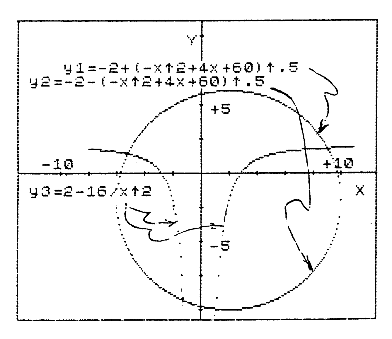

   5 REM ** "G-14", 7-22-89, [illegible]
  10 REM ** PLOTTING EQUATIONS
            with TWO RADICALS
  20 PLOT 0,86: DRAW 0,-86: DRAW
 255,0: DRAW 0,86: DRAW -255,0:
DRAW 0,89: DRAW 255,0: DRAW 0,-8
9: PLOT 130,0: DRAW 0,175
  40 FOR n=6 TO 166 STEP 20: PLO
T 129,n: PLOT 131,n: NEXT n
  50 FOR n=30 TO 230 STEP 20: PL
OT n,87: PLOT n,85: NEXT n
  60 PRINT AT 1,15;"Y";AT 10,30;
"X"
  70 PRINT AT 1,17;"+10";AT 20,1
7;"-10": REM ** SCALE, Y-AXIS
  80 PRINT AT 10,2;"-10";AT 12,2
7;"+10": REM ** SCALE, X-AXIS
 100 LET V=8: LET H=10
 120 FOR x=-2 TO +10 STEP .1
 130 REM ** FIRST CURVE
 140 LET radical=8-x
 150 IF radical<0 THEN GO TO 220
 160 LET y1=+2*radical↑.5
 170 LET y2=-2*radical↑.5
 180 IF ABS y1*V>86 THEN GO TO 2
00
 190 PLOT x*H+130,y1*V+86
 200 IF ABS y2*V>86 THEN GO TO 2
20
 210 PLOT x*H+130,y2*V+86
 220 REM ** SECOND CURVE
 230 LET radical=x-1
 240 IF radical<0 THEN GO TO 295
 250 LET y3=1+radical↑-.5
 260 LET y4=1-radical↑-.5
 270 IF ABS y3*V>86 THEN GO TO 2
85
 280 PLOT x*H+130,y3*V+86
 285 IF ABS y4*V>86 THEN GO TO 2
95
 290 PLOT x*H+130,y4*V+86
 295 NEXT x
 300 PRINT AT 3,1;"y1=+2(8-x)↑.5
"
 310 PRINT AT 5,1;"y2=-2(8-x)↑.5
"
 320 PRINT AT 13,1;"y3=1+(x-1)↑-
.5"
 330 PRINT AT 15,1;"y4=1-(x-1)↑-
.5"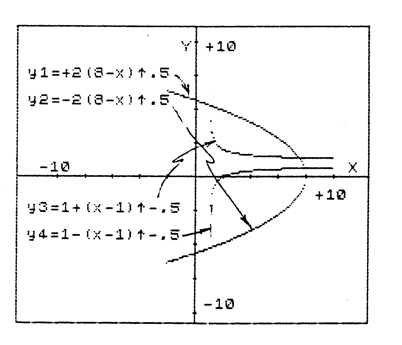

There are simplier ways of plotting these curves, but the method used here allows us to suggest a means of solving these equations simultaneously, using the computer to do the heavy, tiring computations. It involves computing the common x and y values at their points of intersection. This will be the subject of some future tutorial. Hang in there…..

Warren Fricke