A Fast Well-Behaved Pattern Flood Fill

Recursion has always held a certain fascination for me because it seemed that it made very complex problems solvable with a simple, almost magical step. I have written about recursion before in a back issue of ZQA! so I won’t be rehashing that material here, but a brief review is in order before we tackle the subject of flood fills.

A Review of Recursion

So what exactly is recursion? In simplest terms a recursive algorithm is one that calls itself. One class of recursive algorithms breaks a complicated problem into smaller, simpler pieces and then repeatedly applies itself to those pieces, breaking them down even further. Eventually, if everything goes well, you will wind up with many small problems that can be trivially solved. An example of a recursive algorithm of this class is a recursive solution to the Towers of Hanoi problem or the Quicksort sorting algorithm. Another class of recursive algorithms makes use of recursive backtracking — a complex problem is solved by trying to solve it one step at a time. When a step is taken that cannot lead to a solution, the algorithm backs off and tries another step. Recursive algorithms in this class include solutions to the Eight Queens problem and the Knight’s Tour problem. You can find recursive solutions to the Towers of Hanoi and Knight’s Tour written in BASIC in a back issue of ZQA!.

For those of us without back issues of ZQA! handy, let’s investigate the one recursive algorithm that everyone sees in Computer Science 101 ~ the computation of a factorial. N! (N factorial) is defined as (N)x(N-l)x(N2)x. ..xl with N being a positive integer. 5! = 5x4x3x2x1 = 120, for example. 0! is defined as 1. A recursive solution might look like this:

    int factorial (int n) 
    {
       if (n <= 1)
         return 1; 
       return n*factorial(n-1);
    }

Wait a minute, that’s not a BASIC subroutine, that’s a C function! Sinclair BASIC does not directly support recursion so a BASIC version of the above would need a bunch of artifacts decorating it which would only obscure the point I want to make. Now that a decent C compiler is available for our T/S machines, I don’t feel too guilty about sticking with the C. We make a call, asking to compute the factorial of N. If N <= 1 the answer is 1 (ignoring the case that N is negative which should throw an error). Otherwise the problem is too difficult to solve so it is broken into a smaller one: N times the factorial of (N-1).

That was easy, but it might be initially surprising to learn that this is a poor method for calculating factorials. To understand why, we’ll need to pay closer attention to what is involved in a recursive call. The factorial function, as written above, needs to remember two things: the number N and where it was called from so that it can return there later. Compiling the above for a TS-2068 using the z88dk C compiler would reserve two bytes to store N and two bytes for the return address, for a total of four bytes. So the initial call to compute 5! would require four bytes to be reserved. But then factorial(5) would try to return “4*factorial(4)”, causing another call to be made to factorial with N=4, requiring another four bytes. Factorial(4) would make a call to factorial(3), requiring a further four bytes, etc. In other words, to find the answer to factorial(5), the computer would make calls to factorial(5), factorial(4), factorial(3), factorial(2) and factorial(l). Factorial(I) returns 1 as the answer, factorial(2) returns 21 as the answer, factorial(3) returns 3*2 as the answer, factorial(4) returns 4*6 and factorial(5) returns 5*24. We say that factorial(5) has a recursion depth of 5 because a maximum of five instances of factorial will exist at any one time during its computation. With each instance needing four bytes to remember its value of N and return address, factorial(5) requires 5*4=20 bytes of memory to compute the result. More generally we can say that the recursion depth of factorial(N) is N and 4*N bytes are required to compute the result.

Even on our small 64K machines, that doesn’t seem to be a lot of memory and really it isn’t. Things get worse if you try to compute something like 69! which would seem to require 276 bytes in the recursive solution. I say “seem to” because we would need a new large variable to hold the result in each recursion step — 69! requires 41 bytes to hold its value precisely! Switching to a floating point representation would reduce that to four bytes (at the expense of precision), compared to the two bytes we’ve assumed (the result in each step is held in the HL register pair, a consequence of how the z88dk C compiler does things). With the way our subroutine is written now we couldn’t compute anything more than 8! and therefore memory 7 usage is never really an issue. Other recursive algorithms may have a recursion depth in the thousands with dozens of bytes needed for each instance. Then the matter of memory is significant, and, indeed, you will see one such example shortly.

Another problem with the factorial recursive solution in our case is runtime. It takes time to set up calls and return from them – these actions translate directly into pushes and pops on the Z80’s stack. Compare this recursive solution to the “regular” iterative solution below:

int factorial (int n)
{
   int fact, i; 
   fact = 1 ;
   for (i=2; i<=n; i++)
       fact = fact*i; 
   return fact;
}

We need two bytes for “fact”, two bytes for “i”, two bytes for “N” and two bytes for the return address = 8 bytes total no matter what “N” is. There are no calls to set up, just a for loop. This version will be faster and use up a small, fixed and predictable amount of memory. It is superior to the recursive solution in every way.

So what is the conclusion of all this discussion? You must use recursion with care. It can be a panacea to solve many very difficult problems, but you must be fully aware of how much memory will be required and the rantime necessary in comparison to an equivalent iterative solution. The Towers of Hanoi solution in a back issue of ZQA! has a maximum recursion depth of 64 (for 64 disks) and the Knight’s Tom has a recursion depth of 64 (the number of squares on a chess board), very manageable numbers. You can see in both of those BASIC solutions that an array of those sizes was allocated to remember the state in each recursive step.

A Recursive Flood Fill Algorithm

So what has all this got to do with flood filling? It turns out that the obvious approach to filling an arbitrary region involves a recursive solution. And the recursive solution is a bad one.

In comp.sys. Sinclair, Geoff Wearmouth shared a BASIC subroutine from an early ’80s type-in magazine that would fill an arbitrary area on screen bounded by a solid pixel boundary. Here it is:

    5 REM AUTHOR UNKNOWN
   10 CIRCLE 128,88,4
   20 LET X=100 : LET Y = 100 : REM START POINT
   30 GO SUB 1000 : STOP
 1000 PLOT x, Y 
 1010 IF NOT POINT (X+1,y) THEN LET x=X+1 : GO SUB 1000 : LET x=x-1
 1020 IF NOT POINT (x-1,y) THEN LET x=x-1 : GO SUB 1000 : LET x=x+1
 1030 IF NOT POINT (x, Y+1) THEN IET y=y+1 : GO SUB 1000 : LET y=y-1 POINT (X, Y-1)
 1040 IF NOT POINT (x, Y-1) THEN LET y=y-1 : GO SUB 1000 : LET y=y+1
 1050 RETURN

The main subroutine begins at line 1000 and the algorithm used is a recursive one (did you spot the “GOSUB 1000” statements in the subroutine itself?) Filling an arbitrary region is not a trivial problem so a recursive approach is taken to whittle away all the complexity. The fill subroutine above plots the current point (the PLOT on line 1000) and then tries to move in all four directions away from the point. Before each move, it checks to see if the point is already black, indicating a boundary. If not, it considers it a valid move and tries to fill from that point by calling itself with the new pixel coordinate in (x,y).

Earlier I mentioned that Sinclair BASIC does not directly support recursion. The reason it doesn’t can be seen in this fill program Each run through the subroutine at 1000 expects to have its own private copy of (x,y). The value of (x,y) at 1010 must be the same value at line 1020, 1030 and 1040 in order for the program to work. But there are one or more “GOSUB 1000” calls in the middle, which themselves require new values of (x,y) and which will themselves change (x,y). Sinclair BASIC has only one copy of these variables which must be shared by each recursive call. A recursive C call would give each “GOSUB” a private copy of (x,y) on the stack independent of all other “GOSUBs”. ‘ Not so* in Sinclair BASIC, So the problem is, after each “GOSUB 1000” in the fill subroutine, how do we make sure that our own (x,y) has not changed? In the above code, the solution is simple. We promise that when “GOSUB 1000” returns, the value of (x,y) is not changed from what it was when “GOSUB 1000” was executed. In line 1010, for example, x is increased by one before a call to “GOSUB 1000”. Because of our promise (the jargon calls such a promise an “invariant”) we know that when the GOSUB returns, x will be one larger than what it was at the beginning of line 1010. So to get x back to where it was, decrease by one and everything will be fine for the next line. Before the routine returns in line 1050 we know that (x,y) has not changed from its initial state in line 1000. That’s the subroutine keeping its promise.

The kind of fill algorithm this program uses is formally called a flood fill because the fill “floods away” from the initial point in all directions. Other fill algorithms exist, but this one is both easy to understand and capable of filling any arbitrary region without restrictions. Earlier I hinted that a recursive solution to the flood fill problem is a bad one. I’ll leave that thought here and come back to it later when we’ve looked at a couple of machine code implementations of the algorithm. For now, realize that each “GOSUB” requires the TS-2068 to remember a return line number (two bytes) and then consider what the recursion depth might be for a 256×192 resolution blank screen (hint – you wouldn’t be far off if you just multiplied 256 and 192 together!).

ff you typed in the BASIC program and ran it you’d realize that it is mighty slow. Any useful fill utility will need to be written in machine code. To do that, we will need to review the structure of the TS-2068’s display file.

Display File Organization

The TS-2068’s display file is where all the screen information is stored. The SCLD chip constructs the TV display by reading the information stored there. The display file is termed “memory-mapped” because the storage exists in the z80’s memory space, from address 16384 to 22527 (not counting the colour attributes for each character). If you poke values into those addresses you will see the display change. In the TS-2068’s other display modes (dual screen, hi -colour, hi-res) more areas of memory are used to hold the display. In tins article, we’ll only concern ourselves with the default 256×192 mode.

A pixel display occupying 16384 to 22527 reserves 6144 bytes to store all the screen information. The TS-2068 has a resolution of 256*192 = 49152 pixels. How do we cram information about 49152 pixels into 6144 bytes? Well, each pixel can be represented by one bit – either one or zero, on or off. Cramming 8 pixels into a byte, we’d need 256*192/8 – 6144 bytes. Problem solved!

A simple way to organize the display might have pixels 0..7 for the top line of the display stored at address 16384, pixels 8..15 at address 16385,… pixels 248-255 stored at address 16415. The next pixel line would follow with pixels 0.. 7 of line 1 at address 16416, and so forth for all 192 lines on the screen. This is indeed how the TV draws its display, left to right, top to bottom. But the display organization was chosen to optimize the printing of characters so it’s not done in this simple manner. To see evidence of this, try this short program:

  10 FOR z=16384 TO 22527
  20 POKE z,255
  30 NEXT z

If you run this program you will witness how the display file is organized. On the largest scale you will notice that the display is divided into three parts (called blocks). First the top block is filled- then the second and finally the third. Each block is further divided into eight character lines. Each of these lines is divided into eight scan lines. The first scan line for all character lines in a block is filled, followed by the second scan line for all character lines, all the way to the final eighth scan line. Each scan line itself is composed of 32 horizontal bytes with each byte holding eight pixels.

This organization sounds complicated but it really isn’t that bad if some thought is applied to it. By paying attention to how the display is built up in increasing byte order (reread the paragraph above), we can construct a screen address given block, character line, scan line and column as follows:

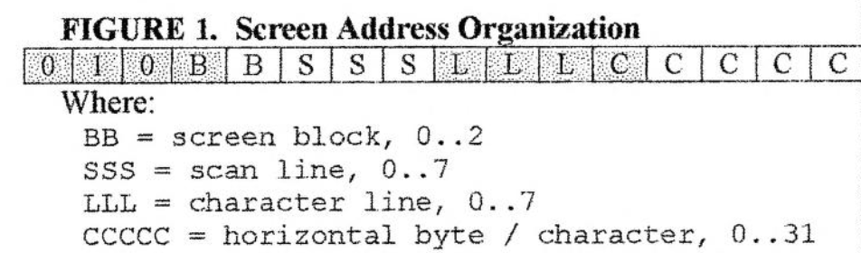
While observing the BASIC program, you’ll notice that the horizontal column changes the fastest. There are 32 columns, requiring 5 bits to represent those. They increase the fastest so they appear in the bottom 5 bits of the 16-bit address. The next fastest tiring that changes is the character line. There are 8 lines in each block, requiring 3 bits to represent them. These 3 bits appear next to the column bits. Next, in order of fastest changing, are the scan lines (8 of them requiring 3 bits) followed by the block (3 of them requiring 2 bits). The display starts at address 16384 (0x4000) so we add that to our 16-bit address. This is responsible for the lone T you see in figure 1.

The character position row = 10, column = 12 is located in block 1 (the second block since it holds the second third of the display, rows 8.. 15), line 2 (the third character line in this block ~ rows 8, 9, 10), scan lines 0 (top) through 7 (bottom) for the full character square, and column 12. This leads to a screen address that looks like:

To print a letter ‘A’ at (10,14), poke the appropriate values into memory at these addresses:

 POKE 18508, BIN 00000000
 POKE 18764, BIN 00111100
 POKE 19020, BIN 01000010
 POKE 19276, BIN 01000010
 POKE 19532, BIN 01111110
 POKE 19788, BIN 01000010
 POKE 20044, BIN 01000010
 POKE 20300, BIN 00000000

At this point you may realize why UDGs and printed characters are 8×8 pixels in size. There are 8 vertical scan lines in each character line and there are 8 pixels packed into a byte. But you may not realize why this particular display file organization speeds up character printing. If you back up and look at the screen addresses computed above, you’ll notice that each scan line is separated by 256 bytes (you could also see this from figure 1). In assembly language, an address is held in a register pair, like HL. Adding 256 to an address is a quick matter of incrementing the most significant register, in this case H with the “INC H” instruction. That’s all it takes! Moving horizontally to the right one character position involves adding one to the screen address, which can be done just as quickly with “INC L”. You can’t get any faster than that. In fact, this display file organization was patented by Sinclair’s Richard Altwasser back in 1982.

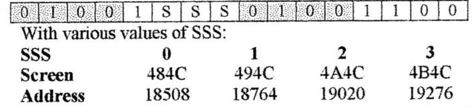
That’s all fine and good but we still haven’t managed to easily map a pixel coordinate to a screen address. Here’s how we do it:

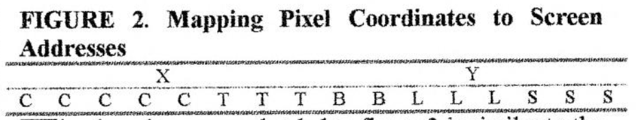
The thought process that led to figure 2 is similar to the previous one. The X coordinate is more or less obvious: there are 32 columns horizontally (5 bits) with each column containing 8 pixels (requiring 3 bits). The pixel position within a byte (0..7) changes fastest as we move horizontally so it appears as “TTT” in the least significant bits of X. For the Y coordinate, the fastest changing item as we move from the top of the screen to the bottom is the scan line, followed by the character line, followed by the block.

Given an X coordinate in the range 0-255 and a Y coordinate in the range 0-192, convert them to binary as in figure 2 and reassemble the bits as in figure 1. For example, pixel coordinate (x.y) = (133,67) in binary is (1000 0101, 0100 0011) with CCCCCM0000, BB=01, LLL=000, SSS=011 according to figure 2. Moving the bits around to the form in figure 1 gives an address of “0100 1011 0001 0000” or 19216 in decimal. The bits “TTT” in the X coordinate do not appear in figure 1. They identify which bit within the screen byte corresponds to the individual pixel. “0” corresponds to the leftmost bit and “7” corresponds to the rightmost: in this case it’s 5. To plot the pixel (133,67) we could simply “POKE 19216,BIN 00001001).

If this had to be done by hand for each pixel, it would get tedious quickly. Here’s a short machine code routine that follows this procedure:

; Get Screen Address 
; 
; Returns the screen address and pixel mask corresponding 
; to a given pixel coordinate. 
; enter: a = h = y coord 1 = x coord 
; exit : de = screen address, b = pixel mask 
; uses : af, b, de, hl 
.SPGetScrnAddr
   and $07        ; A = 00000SSS
   or $40         ; A = 01000SSS
   ld d,a         ; D = 01000SSS
   ld a,h         ; A = Y coord = BBLLISSS
   rra
   rra
   rra            ; A = ???BBLIL
   and $18        ; A = 000BB000
   or d           ; A = 010BBSSS
   ld d,a         ; D = 010BBSSS top 8 bits of address done 
   ld a,1         ; A = X coord = CCCCCTTT
   and $07        ; A = 00000TTT
   ld b,a         ; B = 00000TTT = which pixel?
   ld a, $80      ; A = 10000000
   jr z, norotate ; if B=0, A is the right pixel so skip 
.rotloop
   rra            ; rotate the pixel right one place B times
   djnz rotloop 
.norotate
   1d b, a        ; B = pixel mask
   srl 1
   srl 1
   srl 1          ; L = 000CCCCC
   ld a, h        ; A = Y coord = BBLLLSSS
   rla
   rla            ; A = LLLSSS??
   and $e0        ; A = LLL00000
   or 1           ; A = LLLCCCCC
   ld e, a        ; E = LLLCCCCC
   ret  0         ; DE = 010BBSS LLLCCCC, the screen address!

The subroutine is called with A=H=Y coordinate and L=X coordinate and we get the screen address in DE and the pixel mask in B on the way out. If we ORed B into (DE), we could plot the pixel. If we ANDed the complement of B into (DE), we could unplot the pixel and if we ANDed B with (DE) we could test whether the pixel was set.

This subroutine is great for calculating a screen address corresponding to a pixel position from scratch, but you’ll notice that it is rather lengthy and therefore slow, in a relative sense. Frequently you’ll be plotting a pixel and then plotting many more nearby, possibly a single pixel away. For example, in the process of drawing a line, the initial point is plotted and then succeeding points above, below, to the left or right are plotted. We could handle the drawing of the line as plotting many individual pixel points, calling the above subroutine to compute the screen address for every pixel, but that would be much slower than working directly on the screen address to move up, down, left and right from a current pixel position.

Let’s investigate further to substantiate that claim Given a screen address in HL and a pixel mask in B, how would one move left one pixel? Here’s the necessary code:

; h1 = screen address, B = pixel mask
.left 
  rlc b
  ret nc
  dec 1
  ret

The pixel mask is rotated left one bit. This will be a valid pixel position unless B was already at the leftmost pixel position in the screen byte (i.e. B=1000 0000). The “RLC B” instruction will set the carry flag in that case and leave B=0000 0001. We use the no carry flag to return early if the new screen address and mask is valid, otherwise we update the column position one character to the left (the “CCCCC” portion of the screen address in figure 1). The value of B at this point is 0000 0001, correctly masking the rightmost pixel in the new screen byte to the left of the old one. These four instructions are clearly quicker than rerunning the screen address subroutine. The right pixel movement is similar, substituting “rrc b” for “rlc b” and “inc 1” for “dec 1”. Notice that these subroutines don’t check if we run off the edge of the screen on the left or right side.

To move up a pixel, we need to move up a scan line (decrease “SSS” in figure 2). If we wrap past the first scan line (0), we need to decrease the character line. If we move past the first character line (0), we need to decrease the block. Here is the necessary code:

; hl = screen address
.SPPixelUp 
  ld a,h            ; A=H=010BBSSS
  dec h             ; decrease SSS
  and $07           ; if SSS was not originally 000
  ret nz            ; we're done
  ld a, $08         ; otherwise SSS=111 (correct)
  add a, h          ; and we fix BB in H (one was subtracted) 
  ld h, a
  ld a, l           ; A=X coord=LLLCCCCC
  sub $20           ; decrease LLL
  1d l, a
  ret nc            ; if no carry, LLL was not originally 000, okay 
  ld a,h            ; otherwise LLL=111 now, that's okay
  sub $08           ; but need to decrease screen block
  1d h, a ret

Tis subroutine derives a lot of speed by minimizing the number of instructions executed in the most common cases. For example, 7 out of 8 times, only the first four instructions will be executed. 7 out 64 times, the first 1 1 instructions will execute and the rest of the time (1 out of 64) all the instructions will execute. This makes the subroutine much quicker than one would initially guess by looking at the size of the code. The PixelDown subroutine is similar but is not shown here. All these pixel movement routines are reprinted in full in the floodfill listings elsewhere in this article.

That’s enough information to have a first crack at a machine code version of the BASIC flood fill routine.

Machine Code Flood Fills

Figure 3 contains a direct conversion of the BASIC flood fill we saw earlier. No optimization has been done but it has been improved slightly to check for moving across the screen boundary . Type in the associated BASIC listing to see it in action.

We have managed to speed things up considerably by moving to machine code, but there are still a couple of improvements that can be made. First we compute screen addresses for every single point plotted Since we always move up, down, left or right from the current pixel we could speed things up by avoiding this computation as discussed earlier. The other optimization we can make is to plot a Ml 8 pixels at a time rather than one. What? Recall that each screen byte holds eight pixels. Why fiddle with it eight times to plot eight pixels in it when we could plot all 8 pixels at once with a single write of a whole byte?

The secret to plotting multiple pixels at once is the bytefill subroutine. It operates directly on a screen address and pixel mask, exactly what we will have available now that we have decided not to compute the screen address for every single pixel plotted.

; hl = screen address 
; b = incoming pixel mask 
.Bytefill
   1d a,b          ; get pixed mask
   xor (hl)        ; zero out incoming pixels that
   and b           ; run into set pixels in display
   ret z           ; if no pixels left, ret
.bfloop
   ld b, a         ; b = incoming pixels
   rra             ; expand incoming pixel
   ld c, a         ; to the right and left
   ld a, b  s      ; within byte
   add a, a 
   or c
   or b            ; a = incoming pixels wiggled
   1d c, a         ; save in c
   xor (hl)        ; zero out pixels that run into 
   and c           ; set pixels on display
   cp b            ; have pixels changed from last loop?
   jp nz, bfloop   ; keep going until incoming does not change
   or (hl)
   ld (hl), a      ; fill byte on screen
   scf             ; indicate that this was a viable step
   ret

Bytefill is called with a screen address in HL and a pixel mask containing all the “incoming” pixels. The incoming pixels are those pixels from where the flood fill grows in the current screen byte. Previously the flood fill always grew from a single point but not anymore. The origin of the incoming byte will be clear while perusing the second flood fill listing in figure 4.

The Bytefill routine takes the inconiing pixels and “wiggles” them to the left and right trying to grow tliem into blank spaces within the screen byte. It does this until no more growth is possible within the screen byte. It then plots all those pixels and returns.

Putting these ideas into action produces figure 4, a byte-ata-tinie flood fill routine. Type in the BASIC listing to see it in action. This routine is blazing fast; you will not see anything quicker. But, and this is a big but, there is a major flaw in the recursive algorithm that it shares with all the previous fills we have seen so far: the recursion depth is huge.

Consider a flood fill from the bottom left corner of a blank screen. According to figure 4, the first tiling that is done is the fill of the entire screen byte in the bottom left corner Then a move to the right is made and its byte is filled in a recursive call to “fill”. Followed by another right move and fill, then another, until we hit the right edge of the screen. A right move is not possible from the right edge of the screen so a left move is tried from there. That is unsuccessful because it was just filled. An up movement from the right edge is tried, successfully. Now we are at the right edge, one pixel up from the bottom of the screen. The filler fills in the byte and tries a right movement. That’s not possible so it successfully tries a left movement. If this is carried on you’ll notice that, from the bottom left corner of a blank screen, the screen is filled alternately from the left to the right and then from the right to the left as the fill line moves one pixel higher for each scan line filled. You may have noticed that not a single return instruction is executed during the entire screen fill. That is a problem. Each call to fill puts at least 2 bytes on the stack to remember the return address. Since no returns are made for all screen bytes on the screen, there are 6144 calls made to fill without a single return. That’s a recursion depth of 6144! Since at least 2 bytes are saved on the stack for each recursive call, at least 12288 bytes are needed to complete the fill. The situation can be much worse, however. In the worst case movement (up or down) 6 bytes are saved on a recursive call (two for be, two for M and two for the return address). We may need up to 36864 bytes to fill the screen! The truth is somewhere in the middle. Notice mat by moving from a pixel fill to a byte fill we have reduced the depth of recursion by a factor of eight. Still this amount of memory usage is unacceptable for most applications. How can you use a flood fill in your own programs if it’s going to need most of the available memory to complete?

This recursive fill is an example of a depth-first algorithm. It fills an area by going as deep as possible into the area (one call begets another call begets another, etc. without returning). The result is a recursion depth that is proportional to the area of trie screen to be filled. We can rescue the situation by considering another algorithmic approach, known as a breadth-first algorithm. Instead of going as deep as possible into an area, try going wide first. This sounds like a lot of metaphysical talk of questionable value, but the terms “depth-first” and “breadth-first” are bonafide jargon that is used to describe the solution behaviour of many kinds of algorithms.

A breadth-first approach to a flood fill would, instead of going as far into a screen as possible, try to fill all points in the immediate area first. From a starting point all pixels to the immediate left, right, top and bottom are filled. Then for all those adjacent pixels, their immediate neighbours are filled etc. The savings comes from a key observation: once the immediate neighbours of a pixel are filled, there is no need to remember (come back to) the current pixel. Its information can be forgotten. This was not possible in the previous depth-first approaches. As will be seen later, the breadth-first approach will have a “recursion depth” proportional to the circumference of the area being filled, a significant savings.

Figure 3: Pixel Coordinate Flood Fill

; Flood Fill Version 1 
; H = Y coord 0..191, I = X coord 0..255 
.floodl
    push hl                ; save (x, Y) coordinate
    ld a, h                ; GetScrnAddr requires A=H
    call SPGetScrnAddr     ; compute screen address
    pop hl                 ; restore (x,y) in HL
    1d a, (de)             ; byte on screen
    and b                  ; check if this pixel is set
    ret nz                 ; if so, hit boundary so ret
    ld a, (de)             ; get screen byte
    or b                   ; set this pixel
    ld (de), a             ; plot it on screen
.right
    inc l                  ; move pixel coord right
    call nz, floodl        ; if no wrap 255->0
    dec l                  ; restore x coord
.left
    dec l 
    1d a, l
    inc a
    call nz, floodl        ; if no wrap 0->255
    inc l                  ; restore x coord
.up
    dec h
    ld a, h
    inc a
    call nz, floodl        ; if no wrap 0->255
    inc h                  ; restore y coord
.down
    inc h                  ; move pixel coord down
    1d a, h 
    cp 192                 ; if less than 192
    call c, floodl         ; restore y coord
    dec h
    ret

Figure 4: Byte-At-A-Time Flood Fill

; h = y coord, l = x coord
.flood2
   ld a,h
   call SPGetScrnAddr      ; b = pixel mask
   ex de,hl                ; hl = screen address
.fill
   call Bytefill           ; wiggle around incoming pixel mask
   ret nc                  ; if incoming pixels hit boundary, ret
.up
   push hl                 ; save screen address
   call SPPixelUp          ; move up one pixel
   jr c, offscreen1
   push bc                 ; save pixel mask
   call fill               ; try to fill from new screen position
   pop bc                  ; moving up, pixel mask remains same
.offscreen1
   pop hl
.down
   push hl
   call SPPixelDown
   jr c, offscreen2
   push bc
   call fill
   pop bc
.offscreen2
   pop hl
.right
   bit 0,b                ; if first pixel in mask set, try right
   jr z, left
   inc l                  ; move right one byte
   ld a,l
   and $1f
   jr z, offscreen3
   push bc                 ; save current pixel mask
   ld b,$80                ; new incoming mask = leftmost pixel set
   call fill               ; fill from new screen position
   pop bc
.offscreen3
   dec l
.left
   bit 7,b
   ret z
   ld a,l
   and $1f
   ret z
   dec l
   ld b,$01
   call fill
   ret